Intensity map of unfolded spectral weight

The unfolded spectral weight can be visualized by an intensity map that the weight $w$ is smeared out by a Lorentian function:

$$L(k,E) = \frac{w}{(k/\Delta_k)^2+(E/\Delta_E)^2+1},$$

where $k$ and $E$ are the magnitude of ${\bf k}$-vector in Bohr$^{-1}$ and energy in eV, respectively, and $\Delta _k$ and $\Delta _E$ are the corresponding degree of smearing. Note that the absolute value of the intensity map does not have physical meaning. The visualization can be performed by the following three steps:

(1) Compilation of intensity_map.c

In the the directory 'source', please compile 'intensity_map.c' as

  gcc intensity_map.c -lm -o intensity_map

and copy the executable file 'intensity_map' to your work directory.

(2) Generation of the intensity map

After finising the unfolding calculation, you can generate a file storing a mesh data for drawing the intensity map using 'intensity_map'. For the case of SiC ($2\times 2$) supercell in a two-dimensional honeycomb structure with a Si vacancy discussed in the previous subsection, where the input file is 'SiC_C_SP_V.dat', e.g., one can generate a file 'sic-intmap.txt ' storing the mesh data by

  ./intensity_map sic_c_sp_v.unfold_totup -c 3 -k 0.1 -e 0.1 -l -10 -u 6 > sic-intmap.txt

where the arguments have the following meaning:

  -c     column of spectral weight you analyze
  -k     degree of smearing (Bohr^{-1}) in k-vector                                                                      
  -e     degree of smearing (eV) in energy                                                                            
  -l     lower bound of energy for drawing the map                                                                         
  -u     upper bound of energy for drawing the map

You might be confused by the argument '-c' specifying the column number in the file. When you analyze 'System.Name.unfold_orbup(dn)', you will refer the sequence number for pseudo-atomic orbitals in 'System.Name.out'. Then, it should be noted that the number $N_{\rm col}$ specified by '-c' is related to the sequence number $N_{\rm seq}$ for pseudo-atomic orbitals in 'System.Name.out' by $N_{\rm col}=N_{\rm seq}+2$.

(3) Drawing of the intensity map

Using gnuplot you can draw the intensity map. For example, for the calculation with the input file 'SiC_C_SP_V.dat' it can be done as follows:

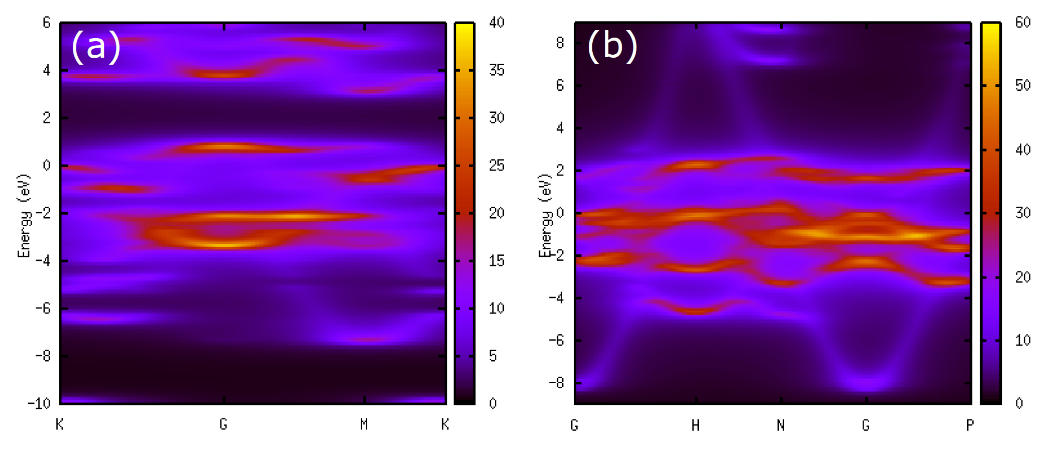
  gnuplot> set yrange [-10.000000:6.000000]
  gnuplot> set ylabel 'Energy (eV)'
  gnuplot> set xtics('K' 0.000000,'G' 0.722259,'M' 1.347753,'K' 1.708883)
  gnuplot> set xrange [0:1.708883]
  gnuplot> set arrow nohead from 0,0 to 1.708883,0
  gnuplot> set arrow nohead from 0.722259,-10.000000 to 0.722259,6.000000
  gnuplot> set arrow nohead from 1.347753,-10.000000 to 1.347753,6.000000
  gnuplot> set pm3d map
  gnuplot> sp 'sic-intmap.txt'

Then, you may obtain a figure as shown in Fig. 52(a).

Figure 52: (a) Intensity map of the unfolded total spectral weight for the up-spin state of a SiC ($2\times 2$) supercell in a two-dimensional honeycomb structure with a Si vacancy, where the SCF calculation was performed by 'SiC_C_SP_V.dat' with a modification that the keyword 'Unfolding.desired_totalnkpt' is set to 300 for better resolution. The degree of smearings are 0.1 (Bohr$^{-1}$) and 0.1 (eV) for $\Delta _k$ and $\Delta _E$, respectively. (b) Intensity map of the unfolded total spectral weight of the cubic cell of Fe in the BCC structure with structural disorder, where the SCF calculation was performed by BCC_Fe_N_SO_Disorder.dat with a modification that the keyword 'Unfolding.desired_totalnkpt' is set to 300 for better resolution. The degree of smearings are 0.1 (Bohr$^{-1}$) and 0.1 (eV) for $\Delta _k$ and $\Delta _E$, respectively.